General remarks
- A lot of functionality is accessible via context menus: use
right mouse-click. - Try dragging some signals from the signals list in Trends to another window.
- Drag-and-drop files from your system file explorer to another Signal Analysis window.
- ASZ- and BDZ-files are automatically opened by Signal Analysis when opening them in your system file explorer.
- Settings are stored in an XML file in the user's profile AppData directory.
Trends
Trends is the starting point of Signal Analysis. You can view your signals, zoom in, hide, scroll through time, and more.
Getting started
Get started by having some signals to work with.
- Import signals from external sources, see Importing signals.
- Use the mouse in the trend axes to zoom
mouse drag up/downand panmouse drag left/down. - Experiment with entries in the
Viewmenu. - Plot one signal versus another signal, see XY Analysis.
- Create a 3D histogram, see 3D Histograms.
Importing signals
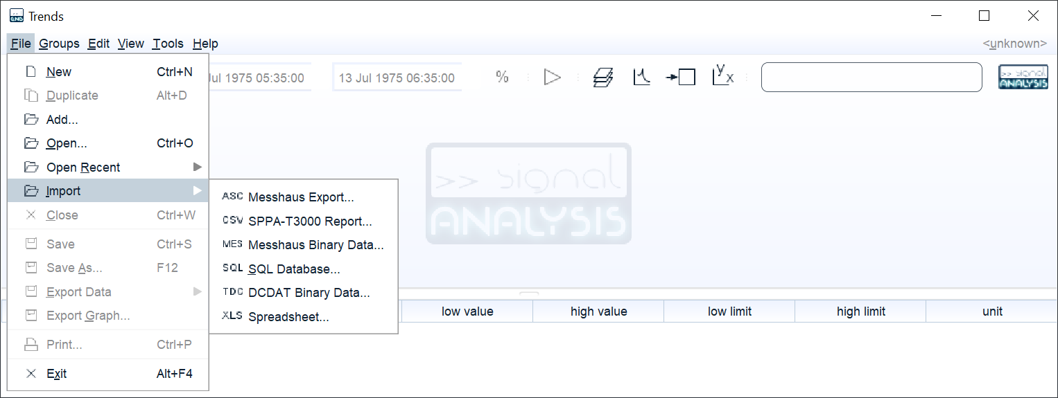
Signals can be imported from external sources like DCS (a plant control system like Siemens SPPA-T3000) output, spreadsheets, a database. The screenshot shows the Import menu. An easy way to import a file is by using drag-and-drop.
Importing signals may show a dialog in which you can select which signals to import and, optionally, apply unit conversions.
Annotations
Signals can be annotated. An annotation is a marker in time that is attached to a signal, like a textual remark or a time frame denoting some event. Annotations are presented graphically in the Trends axes via View > Annotations menu or Alt+A key combination.
You may encounter the following annotations:
Pointa single point in timeLinka link between two or more points in timeBanda band containing all signal values within a time rangeCurtaina period containing all signal values within a time rangeTexta text label, similar to a tool tip
The Annotated Signals File Format
A signal consists of two or more samples. Each sample consists of a timestamp and a value. A sample value can be any real number, either finite, infinite (∞), or not-a-number (NaN).
A NaN value appears when dividing zero by zero.
When a NaN is involved in a mathematical operation, the result is NaN.
When a signal contains a sample with a NaN value, the Trends window draws the line up to the previous finite sample and draws a new line starting from the next finite sample, causing NaNs to appear as gaps.
To obtain the presence of NaNs, the Trends window has a menu to add annotations at the locations of NaNs: Edit > Add NaN Annotations.
A signal also contains meta data like its quantity and unit, a tag and a description. Signals can also contain annotations.
When all timestamps of a signal are an equal time step apart, the signal is said to have a fixed time step, i.e., it's time vector is monotonically increasing.
Signals are stored with file extension ASZ, a custom-made file format optimised for small memory footprint. One ASZ file can contain multiple annotated signals. Normally, sample values are stored in 64 bit (8 byte) floating point precision. To reduce the file size even further, you can choose to store in 32 bit (4 byte). However, this doesn't reduce the file size by a factor of two, because the data is is compressed (zipped) during the storing process and then there's also the timestamps, meta data and (possibly) annotations. A better way to reduce the file size is to apply data reduction, see Processing a Batch of Signals and the Data Reduction block.
You can make a selection of signals from a single file you want to open via the File > Open... menu.
Working with views
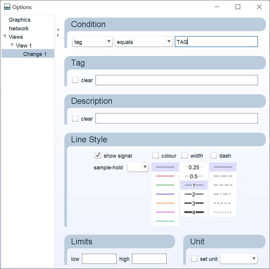
A View is a modification of one or more signals. Views don't actually change signals, Views just change the way signals appear in the Trends window. Views are stored in the user settings file (see Where are user settings stored), not in ASZ files. You can however export these View definitions and store them somewhere for later use, or to import them on another pc.
A View can be used to manually set the Y-axis grid. A View can contain multiple Changes. A Change has a condition which is used to define which signal(s) the change applies to.
XY Graphs
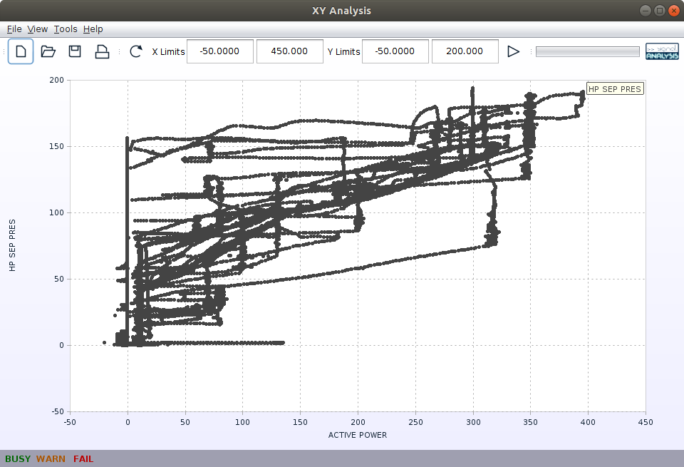
Signals can be plotted against each other via the Tools > XY Graph menu of Trends.
Select two or more signals from the Trends signals list and drag them to an XY Graph window.
Use the mouse to zoom in by selecting a rectangle in the XY axes. Use double-click to reset the zoom level. The tool bar shows current axes limits, which can also be adjusted manually.
3D Histograms

A 3D histogram of the XY data can be created via the Tools > 3D Histogram menu of XY Graph.
The number of bins in which the axes are divided can be adjusted in the tool bar. The XY axes limits are coupled to the associated XY Graph axes. Hovering with the mouse above the histogram bars shows the numeric value in the tool bar.
The numeric values of the histogram are given in the Table tab.
This table can be exported to an Excel spreadsheet via the File > Export Table… menu.
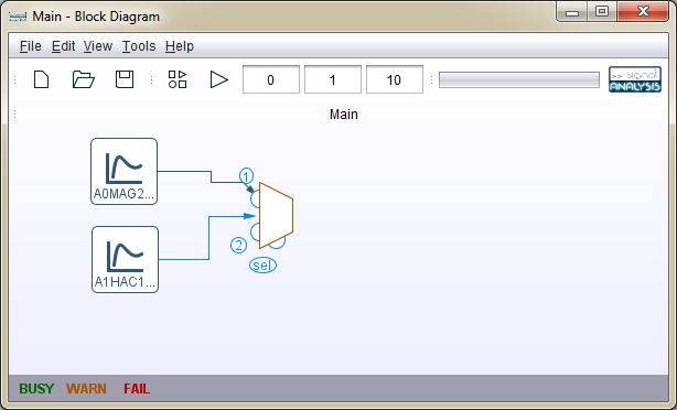
Block Diagrams
You can create a block diagram via the Tools > Block Diagram menu of a Trends window.
In essence, a block diagram consists of a canvas with blocks that interact via connections. Colours are used to give an indication of state: orange for warnings; red for errors; blue for connecting.
The mouse can interact in different ways with the block diagram.
- Hovering above a block shows a tool tip and warning/error messages.
- Clicking on a block selects it. Hold Ctrl to select multiple blocks.
- Clicking on the canvas clears block selections.
- Drag initiated on a block moves the block.
- Drag initiated on the output port of a block initiates making a connection.
- Drag initiated on the canvas shows the selection rectangle.
- Drag while holding Shift moves selected blocks, waypoints, and text areas.
- Right-click shows a context menu.
- Double-click on a block shows the block parameters editing dialog.
Text areas
Multi-line text areas can be added to any location on a block diagram by right-clicking and selecting Add Text Area from the context menu.
To delete a text area, right-click on it and select Delete.
To move a text area, drag while holding shift.
Note that this doesn't work when initiated above a text area since this initiates text-selection.
A text area will automatically resize its width and height to fit its content.
Connecting blocks
Connections can contain either a scalar or a signal.
To connect the output of one block to the input of another, move the mouse to the right-hand side of the source block. When a triangular shape appears, drag the mouse towards the destination block. A candidate connection appears. When the mouse enters a block, the block will show its input ports, sometimes with labels. Release the mouse above the desired input port to make a connection. When released above the block itself, a connection will be made to the first available input port.
Blocks can have multiple input ports but currently only one output port is supported. However, an output port can be connected to multiple destination blocks.
Block input
In general, signals don't have similar timestamps. It is, however, not required to resample block input signals to similar timestamps. A time vector is created which contains the timestamps from all input signals, but limited to the time frame common to all signals. This common time frame prevents extrapolation. Next, all input signals are linearly interpolated at the new time vector and the block operation is performed. As a consequence, performing an operation on multiple signals all with different timestamps, may result in output signals with a lot of samples, resulting in excessive processing times. The Data Reduction block can be used to reduce the number of samples.
Block library
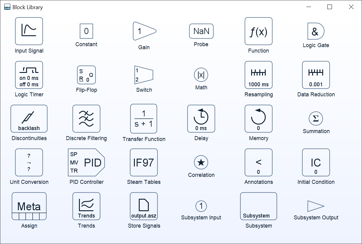
To add library blocks to a block diagram, select one or more blocks from the block library and drag-and-drop them onto the block diagram.
Alternatively, right-click on a block diagram canvas and select Add Block.
Annotations block
This block is used for adding annotations to the entering signal, based on a simple condition.
Assign block
Modifies signal meta data: tag, description, quantity, units, and sample-hold.
Note that this block doesn't modify signal values. For units conversion of values use the Unit Conversion block.
Constant block
Either a scalar constant or a named parameter when this block is part of a Subsystem.
Note that the output of a Constant block doesn't have any associated unit. Use a Probe block to inspect the value of a scalar.
Correlations block
Performs the auto-correlation (single input), cross correlation (two signals), or convolution.
Data Reduction block
Removes samples, from the input signal, which are within the set threshold with respect to neighbour samples.
Delay block
A simple time delay.
Memory block
The memory block outputs the value of the first input at the time of the last high value of the second input. Put in another way, this block stores the value of input 1 in memory when input 2 is high.
Discontinuities block
Simulates backlash, rate limiter, and saturation.
Discrete Filtering block
Supports discrete-time filters moving average (good for noise reduction), low-pass, high-pass, band-pass, and band-reject.
Flip-Flop block
Function block
Maps input values to output values accoring given discrete function profile/table.
Gain block
Multiplies the input signal or constant with given value.
Initial Condition block
Initial conditions are required when there's a circular reference. When the block diagram detects this situation, it switches from explicit mode to implicit mode and will try to solve iteratively.
Please note that implicit mode is currently not fully supported for all blocks.
Input Signal block
Input signal as used in Subsystem blocks.
Logic Gate block
The logic gate block accepts any number of inputs being either constants or signals or a combination thereof. However, the NOT gate only accepts one input being either a constant or a signal and simply inverts its input. The XOR gate outputs 1 if an odd number of inputs are 1. The XNOR gate (which equals a XAND gate) outputs 1 if an even number of inputs are 1.
Note that the order of the inputs does not affect the gate output. Truth tables for two and three inputs are given below.
| input 1 | input 2 | AND | OR | NAND | NOR | XOR | XNOR |
|---|---|---|---|---|---|---|---|
| 0 | 0 | 0 | 0 | 1 | 1 | 0 | 1 |
| 0 | 1 | 0 | 1 | 1 | 0 | 1 | 0 |
| 1 | 0 | 0 | 1 | 1 | 0 | 1 | 0 |
| 1 | 1 | 1 | 1 | 0 | 0 | 0 | 1 |
| input 1 | input 2 | input 3 | AND | OR | NAND | NOR | XOR | XNOR |
|---|---|---|---|---|---|---|---|---|
| 0 | 0 | 0 | 0 | 0 | 1 | 1 | 0 | 1 |
| 0 | 0 | 1 | 0 | 1 | 1 | 0 | 1 | 0 |
| 0 | 1 | 0 | 0 | 1 | 1 | 0 | 1 | 0 |
| 0 | 1 | 1 | 0 | 1 | 1 | 0 | 0 | 1 |
| 1 | 0 | 0 | 0 | 1 | 1 | 0 | 1 | 0 |
| 1 | 0 | 1 | 0 | 1 | 1 | 0 | 0 | 1 |
| 1 | 1 | 0 | 0 | 1 | 1 | 0 | 0 | 1 |
| 1 | 1 | 1 | 1 | 1 | 0 | 0 | 1 | 0 |
Logic Timer block
Math block
Performs common mathmatics operations.
There's operators that work on a single input, like abs (absolute values), and operators the work on multiple inputs.
An input can either be a scalar, i.e. a constant, or a signal.
Switch block
Works as a switch with multiple input ports and a selector port on the bottom.
Output block
Subsystem output.
PID Controller block
Process controller with tracking gain.
Probe block
Useful to see the value of a scalar.
Resampling block
Resamples input signals to a given fixed time step.
Signal block
Signal source reference based on tag and description.
This block doesn't contain a signal, it's merely a reference used to retrieve the signal from the associated Trends window. The associated Trends window is the one from which the current Block Diagram was started. You can bring the associated Trends window to the foreground via Block Diagram's Tools menu.
Steam Tables block
IAPWS-IF97 water/steam properties according the International Association for the Properties of Water and Steam. This is the industrial formulation (faster executing at the cost of a slight loss in accuracy), based on the general/scientific formulation IAPWS-95.
The selected unit system applies to both the input(s) as well as the output. Units of input signals are converted when possible, otherwise an error message is shown. Note that constant inputs (see Constant block) don't have an associated unit and the scalar value is assumed to have the correct unit.
For more information refer to www.if97.software.
Store Signals block
Stores signals (results) to given ASZ file.
Subsystem block
Used for creating Batch Processing blocks.
Subsystems have a list of named parameters for use in, for instance Constant blocks. Subsystems can be nested.
Summation block
The summation block adds up all inputs, either signals or constants, or a combination thereof.
This is just a convenience block which points to the Math block with the add operator.
Transfer Function block
Laplace domain transfer function, currently only supports the following patterns: gain; exponential decay, a/(bs + c); and lead-lag, (as + b)/(cs + d).
Trends block
Sends signals (results) to the associated Trends window.
The associated Trends window is the one from which the current Block Diagram was started and where it looks for input signals as defined by Signal blocks. You can bring the associated Trends window to the foreground via Block Diagram's Tools menu.
Unit Conversion block
Converts units, and values accordingly.
This block can only convert units of like quantities. To change a signal's quantity, use the Assign block.
Frequency Spectra
The Frequency Spectrum tool is for viewing a signal in the frequency domain. The signal is transformed to the frequency domain using the Fast Fourier Transform (FFT) algorithm. The FFT requires a signal with a constant time step, so it will first be resampled to the sample period millisecond setting. The amount of samples used for the transformation, or block size setting, is a power of two, i.e. 2p, where p is a positive integer. By the Nyquist criterion, the selected sample period dictates an upper limit to the frequencies that can be detected. To prevent aliasing, a windowing function (Gauss) is applied to the samples before performing the FFT.
Averaged discrete Fourier transformSpectrogram
Access this tool from Tools > Spectrum menu in a Trends window. Alternatively, press F7 or the tool bar button.
Processing a Batch of Signals
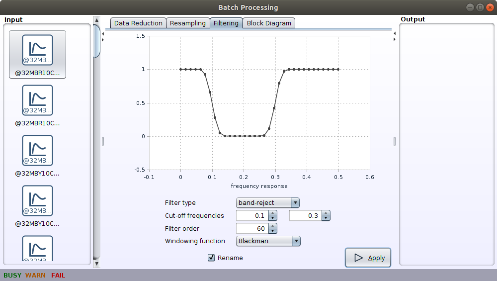
Applying a modification to multiple signals can be tedious when the you need to 'process' a lot of signals.
To aid in this task, you can use the Batch Processing tool accessible via the Tools > Batch Processing menu.
Data Reductionreduce signals to only contain relevant values. For signals with a lot of samples, this can be an essential step to improve handling.Resamplingresample signals to another constant time step.Filteringapply low-pass, high-pass, band-pass, band-reject, and moving average filters.Block Diagramuse your own System Analysis Subsystem block.
Help Dialogs
Help browser
Start the Help browser via the Help > Help menu or by pressing F1.
About dialog
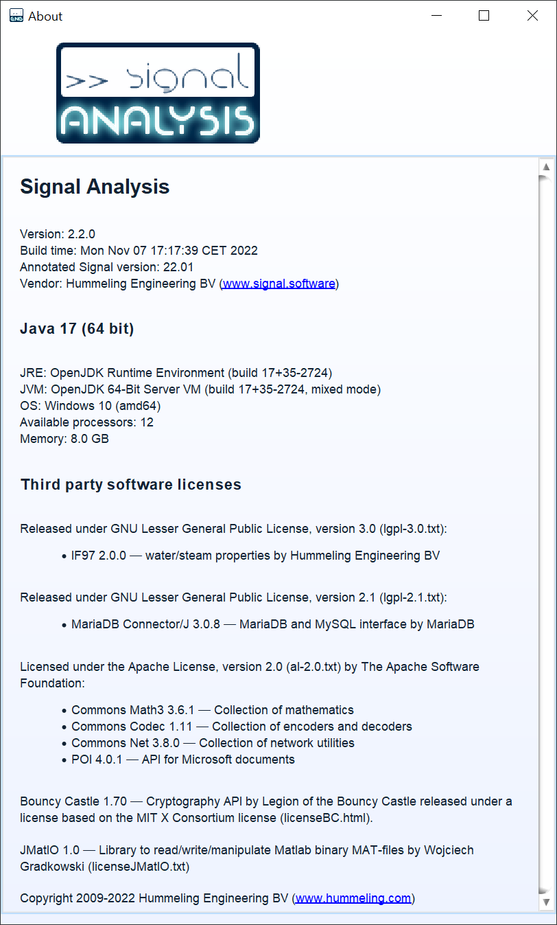
Show the About dialog via the Help > About… menu.
We owe credit to the open-source third party libraries as listed.
Keyboard Shortcuts
| shortcut | action |
|---|---|
| F1 | Help |
| F2 | Rename |
| F3 | Views Panel |
| F5 | Reset Axes (Trends)/Simulate (Block Diagram) |
| F7 | Frequency Spectrum |
| F8 | Block Diagram |
| F9 | XY Graph |
| F12 | Save As… |
| Ctrl+A | Select All |
| Ctrl+C | Copy |
| Ctrl+Shift+A | Select None |
| Ctrl+E | Editing Mode |
| Ctrl+G | Snap To Grid |
| Ctrl+L | Block Library |
| Ctrl+N | New |
| Ctrl+O | Open… |
| Ctrl+P | Print… |
| Ctrl+S | Save |
| Ctrl+T | Options |
| Ctrl+V | Paste |
| Ctrl+W | Close |
| Ctrl+Y | Redo Last Action (Block Diagram) |
| Ctrl+Z | Undo Last Action (Block Diagram) |
| Alt+A | Toggle Annotations |
| Alt+D | Duplicate |
| Alt+L | Toggle Data Lines |
| Alt+M | Toggle Data Markers |
| Alt+P | Toggle Percentage Scale |
| Alt+S | Show All |
| Alt+X | Toggle X Grid |
| Alt+Y | Toggle Y Grid |
| Alt+F1 | Toggle Tool Tips |
| Alt+F4 | Exit |
| Alt+Down | Move divider down (Trends) |
| Alt+Up | Move divider up (Trends) |
| Down | Zoom out (Trends axes) |
| Left | Shift time to the left (Trends axes) |
| Right | Shift time to the right (Trends axes) |
| Up | Zoom in (Trends axes) |
| Shift+S | Toggle Visibility |
| Delete | Delete Selected Signals |
| Page Up | Go To Parent Block Diagram |
Frequently Asked Questions
What is Java heap space
You might encounter a Java heap space exception when working with a lot of data. This is basically telling you that Java exhausted its allocated memory.
Where are user settings stored
User settings, like View definitions and recent files, are stored in your local AppData directory.
This directory resides under your home directory.
Copy-and-paste the following line in Windows Explorer:
%LOCALAPPDATA%\Hummeling\Signal Analysis
In what platform is this app developed
This app is completely developed in Java and uses the following technologies: JavaScript, JSON, XML, HTML, SQL, XLS(X). It is tested on Windows, macOS, and some Debian-based Linux distributions. It uses several open-source third party libraries as listed in the About dialog. The software is distributed from our website: www.signal.software.
How can I contact you
Signal Analysis is developed by Hummeling Engineering BV (www.hummeling.com).
Feel free to contact us when you encounter any difficulties, have a feature request, or when you want to report a bug: engineering@hummeling.com